An atropy tutorial
This tutorial will provide all necessary information to use the functionalities provided by atropy. It helps the user understand how to translate chemical reactions into our implementation and explains some ideas behind our code. We show how to run stochastic simulations of a chemical reaction network by using the Python interface of the atropy code. For that, we show how to setup a model, specify the low-rank algorithm used and run the simulations for the lambda phage example.
The lambda phage model
First we need to take a look at the lambda phage model and its chemical reactions. The lambda phage is a bacteriophage that infects the bacterial species E. coli. and stays dormant in the host or breaks out of the host, after multiplying and reassembling itself. The model consists of 5 species and 10 reactions, each with a corresponding propensity function, visualized in this table:
\[\begin{array}{|c|c|c|} \hline \mu & \text{Reaction } R_\mu & \text{Propensity function } \alpha_\mu(\mathbf{x}) \\ \hline 0 & \star \rightarrow S_0 & a_0 b_0/(b_0 + x_1) \\ 1 & \star \rightarrow S_1 & (a_1 + x_4) b_1/(b_1 + x_0) \\ 2 & \star \rightarrow S_2 & a_2 b_2 x_1/(b_2 x_1 + 1) \\ 3 & \star \rightarrow S_3 & a_3 b_3 x_2/(b_3 x_2 + 1) \\ 4 & \star \rightarrow S_4 & a_4 b_4 x_2/(b_4 x_2 + 1) \\ 5 & S_0 \rightarrow \star & c_0 x_0 \\ 6 & S_1 \rightarrow \star & c_1 x_1 \\ 7 & S_2 \rightarrow \star & c_2 x_2 \\ 8 & S_3 \rightarrow \star & c_3 x_3 \\ 9 & S_4 \rightarrow \star & c_4 x_4 \\ \hline \end{array}\]The coefficients used for the propensity function are given by
\[\renewcommand{\arraystretch}{1.5} % Increase line spacing \begin{array}{|c|c|c|c|} \hline i & a_i & b_i & c_i \\ \hline 0 & 0.5 & 0.12 & 0.0025 \\ 1 & 1 & 0.6 & 0.0007 \\ 2 & 0.15 & 1 & 0.0231 \\ 3 & 0.3 & 1 & 0.01 \\ 4 & 0.3 & 1 & 0.01 \\ \hline \end{array}\]Translate the model to atropy
Before we can begin, we need to import some necessary libraries. Both numpy and sympy are used when generating the initial condition. For plotting, we need matplotlib and atropy_core, the core library of atropy. It gets installed automatically when installing atropy. Lastly, from atropy itself, we import the necessary classes and functions to set up our model and partition and then run the program.
import matplotlib.pyplot as plt
import numpy as np
import sympy as sp

from atropy_core.output_helper import TimeSeries

from atropy import Model, Partitioning, run, species
Before we can set up our reaction system, we need to define the species. For this, the function species from the atropy library is used. In our reaction network for the lambda phage example, there are 5 species. Thus we define
S0, S1, S2, S3, S4 = species("S0, S1, S2, S3, S4")
Next, we need to initialize the model class. To do so, we pass our defined species to the class Model in atropy.
model = Model((S0, S1, S2, S3, S4))
To add our reactions, we do not only need the reaction itself, but also the corresponding propensity function. Thus, we need to define the coefficients used for the propensity functions from our lambda phage reaction network.
a0 = 0.5
a1 = 1.0
a2 = 0.15
a3 = 0.3
a4 = 0.3

b0 = 0.12
b1 = 0.6
b2 = 1.0
b3 = 1.0
b4 = 1.0

c0 = 0.0025
c1 = 0.0007
c2 = 0.0231
c3 = 0.01
c4 = 0.01
Now, let us consider how to translate our chemical reactions to the atropy implementation. For better understanding, we will first consider only two reactions, namely reaction $R_1$ and $R_5$. For reaction $R_1$, our species $S_1$ gets generated from unknown elements. The propensity function is given by $(a_1 + x_4) b_1 / (b_1 + x_0)$. In our code, we exchange $x_i$ for $S_i$. In this way, we do not need to define any more variables. Also note that the propensity function needs to be factorizable. The reaction can be added using the function add_reaction, which is part of the Model class. The first parameter for the function is the reactants, the second the products and the third the propensity function. The propensity function can be passed to add_reaction in factorized form using a dictionary or in a non factorized form. If added in non factorized form, atropy will try to factorize it and report an error, if no factorization can be obtained. We now add reaction $R_1$ to our model:
model.add_reaction(0, S1, {S0: b1 / (b1 + S0), S4: a1 + S4})
Let us now add reaction $R_5$. Here species $S_0$ decays into unknown elements. Our propensity function is given by the law of mass action. Therefore, we can use an abbreviated form and only pass the coefficient instead of the full dictionary for the propensity function:
model.add_reaction(S0, 0, c0)
Adding the full reaction network for the lambda phage example in a clearly structured way can be done as follows:
model.add_reaction(0, S0, {S1: a0 * b0 / (b0 + S1)})
model.add_reaction(0, S1, {S0: b1 / (b1 + S0), S4: a1 + S4})
model.add_reaction(0, S2, {S1: a2 * b2 * S1 / (b2 * S1 + 1.0)})
model.add_reaction(0, S3, {S2: a3 * b3 * S2 / (b3 * S2 + 1.0)})
model.add_reaction(0, S4, {S2: a4 * b4 * S2 / (b4 * S2 + 1.0)})
model.add_reaction(S0, 0, c0)
model.add_reaction(S1, 0, c1)
model.add_reaction(S2, 0, c2)
model.add_reaction(S3, 0, c3)
model.add_reaction(S4, 0, c4)
When we finally added all of our reactions to the model, all left to do is generating the reaction system, using the corresponding function:
model.generate_reaction_system()
Setup the low-rank solver
To set up our low rank solver, we need to take a closer look at our species and the reaction propensities. We want to use a good partition, which reduces the computational complexity of our problem, but still gives accurate results. The idea is to form cuts between dependencies of species in our dependency graph and generate tree structures hierarchically. To understand this better, we will look at the dependency graph of our lambda phage example with some already proposed cuts:
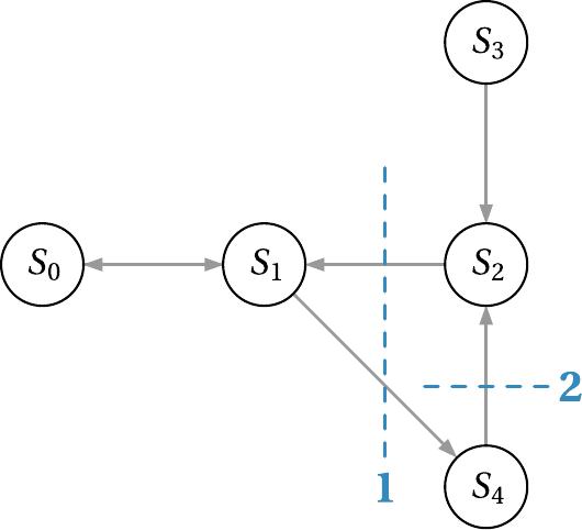
The notation $A \rightarrow B$ indicates the dependency of species $A$ on species $B$ due to some specific reaction propensity. The cuts are chosen in such a way that tightly coupled species are together in the same partition. This selection of cuts results in the following tree structure, where the small numbers at the leaves denote on which species the low-rank factors depend:
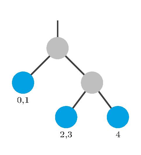
In our implementation, we denote such a structure using a string. Each partition is inside a set of brackets. We give our partition from above the name p0.
p0 = "(S0 S1)((S2 S3)(S4))"
Additionally, we need to set the rank for our calculations. For each partition, the algorithm uses rank $r$ basis functions. The smaller the rank, the faster the calculations are, but we also loose accuracy. For the hierarchical tree structure, we can define the rank for each level, but partitions on the same level use the same rank. This means that we need to assign a rank for each cut of the reaction system and the resulting partitions are approximated to the same degree. In our example, we thus need to define two ranks, which we do in a numpy array in the implementation.
r = np.array([5, 4])
Finally, we can set up our Partitioning class of atropy by passing the partition, array of ranks and the model to our class:
partitioning = Partitioning(p0, r, model)
We have set up our partition, as shown in the first picture. Next, we need to generate the tree, as shown in the second picture. Before doing so, we need to add some grid parameters. Here n denotes the largest population number that we want to track for each species and liml is the lower limit of the population number, which is 0 in our example. The parameter binsize is usually set as in our example. For some problems it might be convenient to group population numbers together to reduce computational effort. Then we can set binsize not equal to 1.
n = np.array([16, 41, 11, 11, 11])
d = n.size
binsize = np.ones(d, dtype=int)
liml = np.zeros(d)
partitioning.add_grid_params(n, binsize, liml)
After we added our grid parameters, we can generate the tree.
partitioning.generate_tree()
Next, we initialize our initial condition class, before assigning a value to it.
partitioning.generate_initial_condition(r)
Setup the initial condition
The initial condition can be arbitrary, but needs to be low rank. Let us consider the already low rank initial condition
\[P(0,x) = \prod_{i=0}^{d-1} f(x_i) \hspace{1cm} \text{with} \hspace{1cm} f(x_i) = e^{-x_i^2}.\]It is even of rank 1, because it can be split into a product of functions, each depending only on 1 species. For this type of initial condition, we provide the function set_initial_condition. It helps the user to translate the information of the initial condition to the nodes of the generated tree. To use it, the function for each species first needs to be written into a dictionary:
functions_dict = {
    S0: sp.exp(-S0**2),
    S1: sp.exp(-S1**2),
    S2: sp.exp(-S2**2),
    S3: sp.exp(-S3**2),
    S4: sp.exp(-S4**2),
}
Now we can call set_initial_condition:
partitioning.set_initial_condition(functions_dict)
To check if the tree and initial condition generation was correct, we can provoke an output in the console. This gives us information about the nodes of our tree.
print(partitioning.tree)
Run the code
Using the run function from atropy, we can finally run our simulation. There are several parameters we need to pass. For the first parameter, we need to pass the partitioning defined above. Next comes the desired output name for the generated files. After that, there is the timestep size and final time of our simulation. The last three parameters are snapshot, substeps and method. They all have a standard parameter, thus only need to be passed if a specific value is desired. The snapshot parameter contains the number of generated output files during our simulation, where the standard value is 2 (i.e. output the initial and final value). The substep parameter is an advanced parameter and for most cases the standard value of 1 should be chosen. For the method, there are 4 different options: implicit_Euler, explicit_Euler, Crank_Nicolson and the standard option RK4. In our lambda phage example, we run the simulation until final time 10 with a timestep size of $10^{-3}$ and implicit Euler, as the time integration method.
run(partitioning, "output_lambda_phage", 1e-3, 10,snapshot=10,
    method="implicit_Euler")
Plot the results
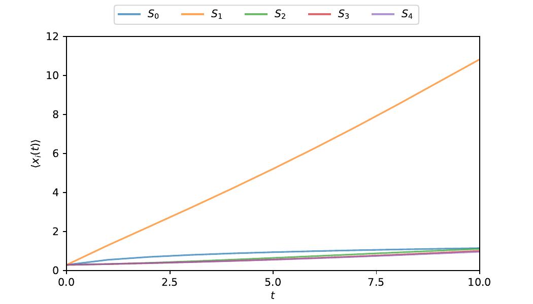
After the simulation has been executed, we can plot our obtained results. To load the generated NetCDF files, the TimeSeries class from atropy_core can be used. In the following, we plot the first moments for each of our species.
time_series = TimeSeries("output_lambda_phage")
concentrations = time_series.calculateMoments()
t = time_series.time

fig, ax = plt.subplots(figsize=(7, 4))

observables = ["S0", "S1", "S2", "S3", "S4"]
observables_alt = ["$S_0$", "$S_1$", "$S_2$", "$S_3$", "$S_4$"]
colors = plt.rcParams["axes.prop_cycle"].by_key()["color"]
for i, (o, o_alt) in enumerate(zip(observables, observables_alt, strict=False)):
    ax.plot(t, concentrations[0][o], "-", label=o_alt, color=colors[i], alpha=0.7)
ax.set_ylabel("$\\langle x_i(t) \\rangle$")
ax.set_ylim([0.0, 12.0])

plt.setp(ax, xlabel="$t$", xlim=[0.0, 10.0],
         xticks=[0.0, 2.5, 5.0, 7.5, 10.0])

lines_labels = [ax.get_legend_handles_labels() for ax in fig.axes]
lines, labels = (sum(ll, []) for ll in zip(*lines_labels, strict=False))
fig.legend(lines, labels, ncols=5, loc="upper center")

plt.savefig("plots/lambda_phage_concentrations.pdf")